Decoding Molecular Complexity: Proudfoot, nSPS, and Assembly Theory
It has been just over a year since I published the first post on this blog, and I still find myself thoroughly enjoying these small investigations. If anything, the questions have gotten more interesting. So - on to another one.
A Year Later, Still Asking: What Is Complexity?
In that first post I looked at the Proudfoot complexity metrics — CM, CM* and Cse — and applied them to a set of recent drug candidates to see where they fell in complexity space. CM* in particular I find intuitive and useful: it is a log-sum of the exponentials of per-atom complexity environments, giving a single number that rewards both diversity and depth of chemical environment.
The question I left hanging was: is CM* the best way to quantify molecular complexity, or is it simply a good one? A year on, there are at least two other frameworks worth putting in the same conversation: the normalized Spatial Score (nSPS) from the Waldmann group, and the much more radical idea of Assembly Theory from Lee Cronin’s group. Both have appeared in the literature within the last few years, and together they illustrate just how unsettled — and how interesting — this area remains.
Why Complexity Is Harder to Define Than You Think
The naive proxy for complexity has long been molecular weight. Bigger molecule = harder synthesis. But this breaks down immediately when you compare, say, polyethylene glycol to strychnine. Both can be large. Only one is genuinely hard to make.
Fsp3 (fraction of sp3 carbons) was introduced as a better proxy, and it genuinely correlates with some useful things — clinical success rates, selectivity, solubility. But Fsp3 is blind to ring topology: a molecule with one sp2 carbon in a strained bridged bicycle will score the same as a flat chain with the same carbon count.
What we really want is a metric that captures the spatial and topological character of a molecule — the things that make a synthetic chemist look at a structure and immediately know it will be a painful target. Two metrics that try to do exactly that are CM* and nSPS.
Coding Workshop: CM* and nSPS Side by Side
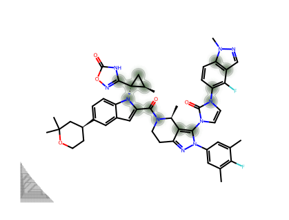
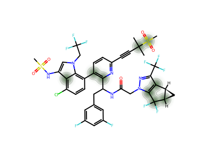
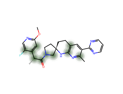
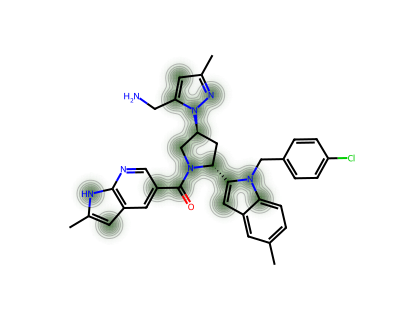
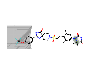
Let’s put both metrics to work on the same set of API structures I used in my first post: RPT193, GDC-0853, Orfoglipron, GS-6207, PF-07258669, compound 14, and PC0371.
First, the imports:
import numpy as np
import pandas as pd

from collections import Counter
from typing import Dict, Iterator, List, Tuple

from rdkit import Chem
from rdkit.Chem import Draw
from rdkit.Chem.SpacialScore import SPS  # built-in since RDKit 2023.09

from matplotlib import pyplot as plt
Now define our compound set — the same one from the molecular complexity post:
data = pd.DataFrame({
    'Name': ['RPT193', 'GDC-0853', 'Orfoglipron', 'GS-6207',
             'PF-07258669', '14', 'PC0371'],
    'SMILES': [
        'ClC1=C([C@@H](C)NC2=NC(N3CC([C@@H]4CN([C@@H]5CC5)C4)CC3)=NC(=N2)N2CCOCC2)C=CC(=C1)Cl',
        'O=C1C(NC2=CC=C(N3[C@@H](C)CN(C4COC4)CC3)C=N2)=C(O)C2=CC=CC=C12',
        'O=C(N1CCC2=NN(C3=CC(C)=C(F)C(C)=C3)C(N4C(N(C5=CC=CC=C5)C(=O)N6CCCC6)=O)=N24)CC1',
        'CC(S(C)(=O)=O)(C)C#CC1=NC(C(CC2=CC(F)=CC(F)=C2)[C@@H]3C[C@@H]4O[C@]5(OC(=O)[C@H]45)CC[C@@H]3F)=CC=C1',
        'CC1=C(C2=NC=CC=N2)C=C(CC[C@]3(CN(C([C@@H](C4=CC=C(F)C=C4)NC(=O)OC(C)(C)C)=O)CC3)O)C=C1',
        'CC(C=C1CN)=NN1[C@H]2C[C@H](C3=CC4=CC(C)=CC=C4N3)C5=CC(=O)N(C6=NC(=CC=C6)C)C25',
        'O=C1NC(C2=CC=C(OC(F)(F)F)C=C2)=NC13CCN(S(CCC4=CC=CC=C4)(=O)=O)CC3'
    ]
})

data
| Name | SMILES | |
|---|---|---|
| 0 | RPT193 | ClC1=C([C@@H](C)NC2=NC(N3CC([C@@H]4CN([C@@H]5C... |
| 1 | GDC-0853 | O=C1C(NC2=CC=C(N3[C@@H](C)CN(C4COC4)CC3)C=N2)=... |
| 2 | Orfoglipron | O=C(N1CCC2=NN(C3=CC(C)=C(F)C(C)=C3)C(N4C(N(C5=... |
| 3 | GS-6207 | CC(S(C)(=O)=O)(C)C#CC1=NC(C(CC2=CC(F)=CC(F)=C2... |
| 4 | PF-07258669 | CC1=C(C2=NC=CC=N2)C=C(CC[C@]3(CN(C([C@@H](C4=C... |
| 5 | 14 | CC(C=C1CN)=NN1[C@H]2C[C@H](C3=CC4=CC(C)=CC=C4N... |
| 6 | PC0371 | O=C1NC(C2=CC=C(OC(F)(F)F)C=C2)=NC13CCN(S(CCC4=... |
Part 1: CM* (Proudfoot Metric)
The CM* metric, originally from Proudfoot (2017), rewards atomic environments that are locally complex — diverse bond paths emanating from each heavy atom. The per-atom complexity CA is:
CA = -Σ(pi·log₂(pi)) + log₂(N)
where pi is the fractional occurrence of each path type and N is the total number of paths from that atom. CM* is then:
CM* = log₂(Σ 2^CA)
Here is the full implementation (carried forward from my first post — it hasn’t changed):
AtomType = Tuple[str, int, int]
Atom = Tuple[int, AtomType]
AtomDict = Dict[Atom, List[Atom]]


def _non_h_items(data: Dict[Atom, any]) -> Iterator[Tuple[Atom, any]]:
    for key, val in data.items():
        if key[1][0] != 'H':
            yield key, val


def _collect_atom_paths(neighbors: AtomDict) -> List[List[tuple]]:
    atom_paths = []
    for atom, nbs in _non_h_items(neighbors):
        paths = []
        for nb in nbs:
            if nb[1][0] == 'H' or neighbors[nb] == [atom]:
                paths.append((atom[1], nb[1]))
            else:
                paths.extend((atom[1], nb[1], nb2[1]) for nb2 in neighbors[nb] if nb2 != atom)
        atom_paths.append(paths)
    return atom_paths


def get_atom_type(atom: Chem.rdchem.Mol) -> AtomType:
    symbol = atom.GetSymbol()
    degree = atom.GetTotalDegree()
    h_count = atom.GetTotalNumHs(includeNeighbors=True)
    non_h = degree - h_count
    return (symbol, degree, non_h)


def fractional_occurrence(data: list) -> np.ndarray:
    counter = Counter(data)
    counts = np.array(list(counter.values()))
    return counts / len(data)


def calculate_cm_star(mol: Chem.rdchem.Mol) -> float:
    """Calculate the CM* molecular complexity metric (Proudfoot, 2017)."""
    atoms = [(atom.GetIdx(), get_atom_type(atom)) for atom in mol.GetAtoms()]
    neighbors = {
        atom: [atoms[neighbor.GetIdx()] for neighbor in mol.GetAtomWithIdx(atom[0]).GetNeighbors()]
        for atom in atoms
    }
    atom_paths = _collect_atom_paths(neighbors)
    cas = np.zeros(len(atom_paths))
    for i, paths in enumerate(atom_paths):
        total_paths = len(paths)
        pi = fractional_occurrence(paths)
        cas[i] = -np.sum(pi * np.log2(pi)) + np.log2(total_paths)
    cm_star = np.log2(np.sum(2**cas))
    return float(cm_star)


def cm_star_from_smiles(smiles: str) -> float:
    try:
        mol = Chem.MolFromSmiles(smiles)
        mol = Chem.AddHs(mol)
        return calculate_cm_star(mol)
    except Exception:
        return np.nan
Part 2: nSPS (Normalized Spatial Score)
The Spacial Score (note: Waldmann’s paper uses this exact spelling, not “Spatial”) was introduced by Ertl, Schuhmann and Waldmann in the Journal of Medicinal Chemistry in 2023. The idea is elegant: assign a numerical score to each heavy atom based on four properties, then sum and normalize by the number of heavy atoms.
For each atom i, the per-atom contribution is:
atom_score(i) = hybridization_score × stereo_score × ring_score × branching_score
where each factor rewards features that make a molecule harder to construct — sp3 hybridization over sp2, stereocenters, non-aromatic ring membership, and higher connectivity. The SPS is the sum over all heavy atoms; the nSPS divides by the heavy atom count to allow comparison across molecules of different sizes.
Since RDKit 2023.09, this is available natively:
from rdkit.Chem.SpacialScore import SPS
Let’s wrap it for our use:
def nsps_from_smiles(smiles: str) -> float:
    """Calculate the normalized Spatial Score (nSPS) using RDKit's built-in module."""
    try:
        mol = Chem.MolFromSmiles(smiles)
        if mol is None:
            return np.nan
        # SPS() returns the raw (unnormalized) spatial score by default.
        # Dividing by the number of heavy atoms gives nSPS.
        sps_value = SPS(mol)
        n_heavy = mol.GetNumHeavyAtoms()
        return sps_value / n_heavy if n_heavy > 0 else np.nan
    except Exception:
        return np.nan
Putting It Together
Now let’s calculate both metrics for our API set and compare:
data['CM*'] = [cm_star_from_smiles(smi) for smi in data['SMILES']]
data['nSPS'] = [nsps_from_smiles(smi) for smi in data['SMILES']]
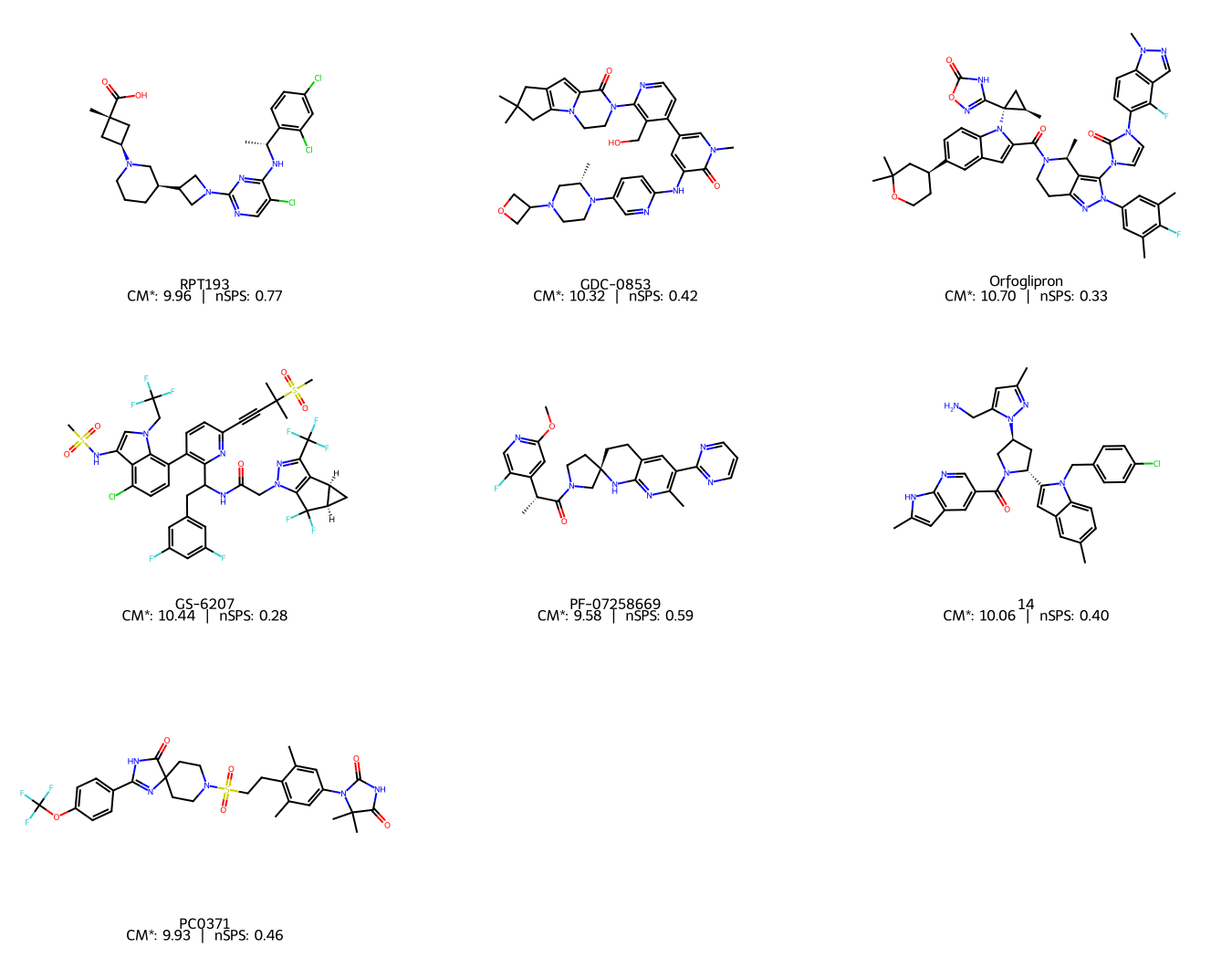
data[['Name', 'CM*', 'nSPS']].round(3)
| Name | CM* | nSPS | |
|---|---|---|---|
| 0 | RPT193 | 9.960 | 0.771 |
| 1 | GDC-0853 | 10.323 | 0.422 |
| 2 | Orfoglipron | 10.702 | 0.333 |
| 3 | GS-6207 | 10.436 | 0.276 |
| 4 | PF-07258669 | 9.577 | 0.590 |
| 5 | 14 | 10.059 | 0.395 |
| 6 | PC0371 | 9.928 | 0.457 |
And visualise the two metrics against each other:
fig, ax = plt.subplots(figsize=(7, 5))

for _, row in data.iterrows():
    ax.scatter(row['CM*'], row['nSPS'], s=60, zorder=3)
    ax.annotate(row['Name'], (row['CM*'], row['nSPS']),
                textcoords='offset points', xytext=(6, 3), fontsize=8)

ax.set_xlabel('CM*  (Proudfoot, 2017)  →  More complex environments')
ax.set_ylabel('nSPS  (Waldmann, 2023)  →  More spatially complex')
ax.set_title('CM* vs nSPS for a Set of Recent Drug Candidates', loc='left', pad=10)
ax.grid(True, linestyle='--', alpha=0.4)
plt.tight_layout()
plt.show()
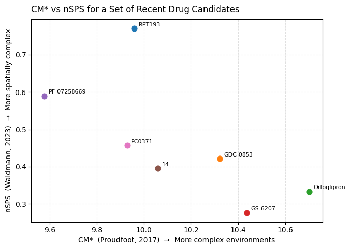
A few things worth noting when you run this:
- Both metrics will place the same molecules in the upper-right corner — the ones with the most intricate ring systems and sp3-rich scaffolds.
- CM* responds strongly to the diversity of atomic environments: a molecule with many different atom types in varied connectivity will score higher even if it is relatively flat.
- nSPS responds more directly to ring membership and sp3 character — it is a more deliberately spatial metric. A bridged bicyclic with four chiral centres but a limited atom-type palette will score relatively higher on nSPS than on CM*.
- Both are normalized by size, which means you are measuring density of complexity, not just raw count. This makes them appropriate tools for design decisions — not post-hoc rationalisation of molecular weight.
Let’s also visualise the structures with their scores annotated, to keep things chemically grounded:
mols = [Chem.MolFromSmiles(smi) for smi in data['SMILES']]

legends = [f"{row['Name']}\nCM*: {row['CM*']:.2f}  |  nSPS: {row['nSPS']:.2f}"
           for _, row in data.iterrows()]

img = Draw.MolsToGridImage(mols, molsPerRow=3, subImgSize=(450, 350), legends=legends)
img
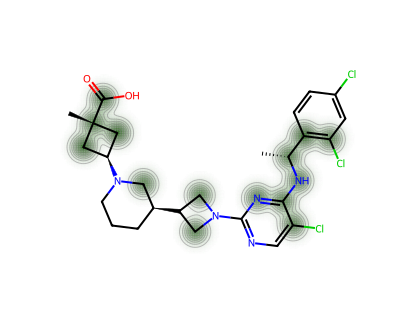
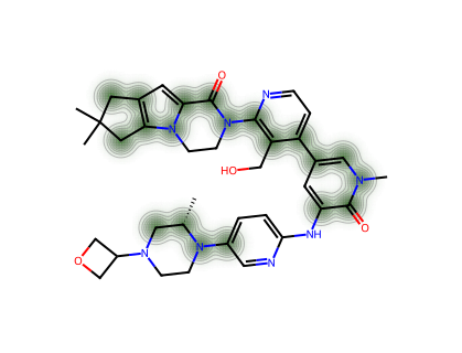
For a single molecule, we can visualise which atoms contribute most to the CM* score.
def atom_complexity_heatmap(smiles: str, threshold: float = 0.8):
    mol = Chem.MolFromSmiles(smiles)
    atoms_list = [(atom.GetIdx(), get_atom_type(atom)) for atom in mol.GetAtoms()]
    neighbors = {
        atom: [atoms_list[neighbor.GetIdx()]
               for neighbor in mol.GetAtomWithIdx(atom[0]).GetNeighbors()]
        for atom in atoms_list
    }
    atom_paths = _collect_atom_paths(neighbors)
    cas = np.zeros(len(atom_paths))
    for i, paths in enumerate(atom_paths):
        pi = fractional_occurrence(paths)
        cas[i] = -np.sum(pi * np.log2(pi)) + np.log2(len(paths))
    cas_norm = (cas - np.min(cas)) / (np.max(cas) - np.min(cas))
    cas_processed = [v if v >= threshold else 0 for v in cas_norm]
    drawer = rdMolDraw2D.MolDraw2DCairo(400, 300)
    SimilarityMaps.GetSimilarityMapFromWeights(mol, cas_processed, draw2d=drawer, alpha=0.2)
    drawer.FinishDrawing()
    bio = io.BytesIO(drawer.GetDrawingText())
    img = mpimg.imread(bio)
    fig, ax = plt.subplots(figsize=(4, 3))
    ax.imshow(img)
    ax.axis('off')
    # Remove all padding/margins so the Cairo image fills the figure exactly
    fig.subplots_adjust(left=0, right=1, top=1, bottom=0)
    return fig
# Heatmap for each compound in the set
for _, row in data.iterrows():
    print(f"--- {row['Name']} ---")
    fig = atom_complexity_heatmap(row['SMILES'])
    plt.show()
--- RPT193 ---
--- GDC-0853 ---
--- Orfoglipron ---
--- GS-6207 ---
--- PF-07258669 ---
--- 14 ---
--- PC0371 ---
The Theoretical Frontier: Assembly Theory
Both CM* and nSPS work on the structure as it is — they measure what it looks like topologically. Assembly Theory asks a different question entirely: how many steps does it take to build this molecule from scratch?
This framework, developed by Lee Cronin’s group at the University of Glasgow and described in a landmark 2021 paper in Nature Communications (Marshall et al., 2021), defines a Molecular Assembly Index (MA) as the minimum number of bond-forming steps required to construct a molecule, given that you can reuse fragments you have already built.
The key insight is deceptively simple. Take any molecule and ask: what is the shortest path to construct it, if you start from individual atoms but are allowed to use any fragment you have already assembled as a building block in a subsequent step? The MA is the length of that shortest path.
This has two remarkable properties:
-
Simple molecules have low MA. Methane (MA = 1) or ethanol (MA ≈ 2) can be assembled in very few steps. Benzene, despite being a sophisticated aromatic system, has a relatively low MA because its high symmetry means the assembly path can reuse the same fragment repeatedly.
-
Biological molecules have high MA. The paper showed that molecules found in living systems — amino acids, nucleotides, secondary metabolites — consistently have MA values above a threshold (~15) that simple abiotic chemistry does not easily cross. This is why the authors propose MA as a potential biosignature for detecting life elsewhere in the universe.
What makes Assembly Theory genuinely different from CM* or nSPS is that it is an information-theoretic measure grounded in construction history, not in the current structure. Two molecules with identical functional groups and similar topology can have very different MA values if one has a highly repetitive substructure (short assembly path) and the other does not.
Practical Access
For those who want to explore MA computationally, the Cronin group has released an open-source Python library:
pip install assembly-theory
This is a high-performance implementation that wraps a Rust backend and is designed to be compatible with RDKit. The original calculation described in the 2021 paper was written in Go (croningp/assembly_go), but the pip package is the most accessible entry point for Python-based cheminformatics workflows.
One important caveat: calculating the exact MA for large drug-like molecules is computationally non-trivial. The assembly space grows rapidly, and the exact minimum path search can be expensive. The pip package implements efficient heuristics, but it is worth being aware of this when working with larger structures.
Summary: Three Lenses on the Same Problem
| Metric | Origin | What it measures | Normalized? | Code availability |
|---|---|---|---|---|
| CM* | Proudfoot (2017) | Diversity & depth of local atomic environments | No (use CM* for relative comparison) | Pure Python / RDKit |
| nSPS | Waldmann (2023) | Spatial & topological character (hybridization, rings, stereo, branching) | Yes (by heavy atom count) | rdkit.Chem.SpacialScore |
| MA (Assembly Index) | Cronin (2021) | Minimum construction steps from atomic building blocks | Context-dependent | pip install assembly-theory |
All three are telling you something about synthetic difficulty, but they are asking subtly different questions. CM* rewards chemical diversity. nSPS rewards spatial architecture. MA rewards informational irreducibility — the idea that a complex molecule encodes a long history that cannot be shortcut.
I find it useful to think of them as complementary rather than competing. Running all three on a candidate structure gives you a richer picture than any single number can. And as always, any number is only as useful as the chemical intuition you bring to interpreting it.
As I said a year ago: please avoid using the word “complexity” without any numbers attached. With Python, RDKit, and a few more tools now at our disposal, there really is no excuse.
As always, the code for this post can be found here.
References
-
Proudfoot, J. R. (2017). A path to improved molecular complexity metrics. Bioorganic & Medicinal Chemistry Letters, 27(9), 2014–2017. https://doi.org/10.1016/j.bmcl.2017.03.008
-
Ertl, P., Schuhmann, T., & Waldmann, H. (2023). Spacial Score: A Comprehensive Topological Indicator for Small-Molecule Complexity. Journal of Medicinal Chemistry, 66(17), 12039–12045. https://doi.org/10.1021/acs.jmedchem.3c01024
-
Marshall, S. M., Mathis, C., Carrick, E., Keenan, G., Cooper, G. J. T., Graham, H., Craven, M., Gromski, P. S., Moore, D. G., Walker, S. I., & Cronin, L. (2021). Identifying molecules as biosignatures with assembly theory and mass spectrometry. Nature Communications, 12, 3033. https://doi.org/10.1038/s41467-021-23258-x
-
Ertl, P., & Schuffenhauer, A. (2023). Molecular Complexity: You Know It When You See It. Journal of Medicinal Chemistry, 66(17), 11902–11904. https://doi.org/10.1021/acs.jmedchem.3c01372
-
assembly-theory Python package: https://pypi.org/project/assembly-theory/
-
Spacial Score GitHub repository: https://github.com/frog2000/Spacial-Score