Molecular Complexity Quantification
I had recently come across a post on LinkedIn discussing the evolution (or chronological increase) of molecular complexity of APIs here.
It immediately struck me that no quantification of moleucular complexity was being shown or quated even though the term was being thrown about heavy-handedly. I posed the question but I got no answer.
I need to say that I have a growing interest in this area and have also published on the the subject of quantifying molecular complexity in a chronological manner, as well as using complexity to predict metrics to guide decision-making in the pharma industry.
So, I did what everyone who is looking for answers and is not getting them would do: I did it myself!
Here is the code and results of my mini-adventure:
First I transcribed the compounds in the post and converted them to SMILES.
Then I calculated the Proudfoot Complexity Metrics for molecular complexity. I find these quite intuitive to use. Additionally, the Python code for calculating them has been published in the second publication given above.
You can find all of the code and supporting data here
#import modules

import numpy as np
import pandas as pd

from collections import Counter
from typing import Dict, Iterator, List, Tuple
from rdkit import Chem
from rdkit.Chem import Draw
from rdkit.Chem.Draw import SimilarityMaps

from matplotlib import pyplot as plt
#"""
#This is the code to calculate the CM, CM_star and Cse metrics.
#Originally developed using Python 3.7, rdkit 2022.3.5, numpy 1.23.2
#"""

AtomType = Tuple[str, int, int]
Atom = Tuple[int, AtomType]
AtomDict = Dict[Atom, List[Atom]]


def _non_h_items(data: Dict[Atom, any]) -> Iterator[Tuple[Atom, any]]:
    """
    Generator for non-H items from a dictionary where the keys are atom tuples.

    Expected keys: (index, (symbol, total degree, non-h degree))
    """
    for key, val in data.items():
        if key[1][0] != 'H':
            yield key, val


def _collect_atom_paths(neighbors: AtomDict) -> List[List[tuple]]:
    """
    Returns list of atom paths for each atom.

    An atom path is a tuple of atom types.
    """
    atom_paths = []
    for atom, nbs in _non_h_items(neighbors):
        paths = []
        for nb in nbs:
            if nb[1][0] == 'H' or neighbors[nb] == [atom]:
                # No second neighbors
                paths.append((atom[1], nb[1]))
            else:
                paths.extend((atom[1], nb[1], nb2[1]) for nb2 in neighbors[nb] if nb2 != atom)

        atom_paths.append(paths)

    return atom_paths


def get_atom_type(atom: Chem.rdchem.Mol) -> AtomType:
    """
    Return a tuple describing the atom type.

    Considers element, total number of connections, and number of non-H connections.
    """
    symbol = atom.GetSymbol()
    degree = atom.GetTotalDegree()
    h_count = atom.GetTotalNumHs(includeNeighbors=True)
    non_h = degree - h_count
    return (symbol, degree, non_h)


def fractional_occurrence(data: list) -> np.ndarray:
    """
    Calculate the fractional occurrence of unique items in the input data.

    Uniqueness determined by collections.Counter.

    Returns:
        np.ndarray: fractional occurrence of unique items
    """
    counter = Counter(data)
    counts = np.array(list(counter.values()))
    return counts / len(data)


def calculate_molecular_complexity(mol: Chem.rdchem.Mol) -> Tuple[float, float, float]:
    """
    This is a function to calculate the CM and CM* molecular complexity metrics described in
    Proudfoot, Bioorganic & Medicinal Chemistry Letters 27 (2017) 2014-2017.
    https://doi.org/10.1016/j.bmcl.2017.03.008

    This function takes an rdkit mol object, identifies the connection paths 1 and 2 atoms away,
    and the calculates the complexity environment for each atom CA as

    CA = - Sum (pi*log2(pi)) + log2(N)

    where pi is the fractional occurrence of each path type emanating from a particular atom and N
    is the total number of paths emanating from that atom.

    Molecular complexity CM can be defined as either the simple sum of the CA,
    or CM* which is the log-sum of the exponentials of the CA.

    CM = Sum (CA)

    CM* = log2(Sum (2**CA))

    Cse = - Sum (qi*log2(qi))

    where qi is the fractional occurrence of an atom (or atom environment).
    """
    # get atom types for each atom in the molecule
    atoms = [(atom.GetIdx(), get_atom_type(atom)) for atom in mol.GetAtoms()]

    # create dict with neighbors of each atom
    neighbors = {
        atom: [atoms[neighbor.GetIdx()] for neighbor in mol.GetAtomWithIdx(atom[0]).GetNeighbors()]
        for atom in atoms
    }

    atom_paths = _collect_atom_paths(neighbors)

    cas = np.zeros(len(atom_paths))
    for i, paths in enumerate(atom_paths):
        total_paths = len(paths)
        pi = fractional_occurrence(paths)
        cas[i] = -np.sum(pi * np.log2(pi)) + np.log2(total_paths)

    cm = np.sum(cas)

    cm_star = np.log2(np.sum(2**cas))

    # sort and concatenate the individual paths to compare the atom environments
    atom_environments = [tuple(sorted((paths))) for paths in atom_paths]

    # Now we can calculate the Cse metric as the fractional occurrence of each atom environment
    qi = fractional_occurrence(atom_environments)
    cse = -np.sum(qi * np.log2(qi))

    return float(cm), float(cm_star), float(cse)


def molecular_complexity(smiles: str) -> Tuple[float, float, float]:
    """This function takes SMILES and returns the CM, CM*, and Cse metrics"""
    try:
        mol = Chem.MolFromSmiles(smiles)
        mol = Chem.AddHs(mol)
        return calculate_molecular_complexity(mol)
    except Exception:
        return np.nan, np.nan, np.nan
#load data

data = pd.read_excel('data.xlsx', header=0)

data
| Name | SMILES | |
|---|---|---|
| 0 | RPT193 | ClC1=C([C@@H](C)NC2=NC(N3CC([C@@H]4CN([C@@H]5C... |
| 1 | GDC-0853 | O=C1C(NC2=CC=C(N3[C@@H](C)CN(C4COC4)CC3)C=N2)=... |
| 2 | Orfoglipron | O=C(N1CCC2=NN(C3=CC(C)=C(F)C(C)=C3)C(N4C(N(C5=... |
| 3 | GS-6207 | CC(S(C)(=O)=O)(C)C#CC1=NC(C(CC2=CC(F)=CC(F)=C2... |
| 4 | PF-07258669 | CC1=C(C2=NC=CC=N2)C=C(CC[C@]3(CN(C([C@@H](C4=C... |
| 5 | 14 | CC(C=C1CN)=NN1[C@H]2C[C@H](C3=CC4=CC(C)=CC=C4N... |
| 6 | PC0371 | O=C1NC(C2=CC=C(OC(F)(F)F)C=C2)=NC13CCN(S(CCC4=... |
Let’s calculate the molecular complexity metrics using the defined functions above
complexity_values = [molecular_complexity(smi) for smi in data['SMILES']]

cm, cm_star, cse = zip(*[tup for tup in complexity_values])

data['CM'] = cm
data['CM*'] = cm_star
data['Cse'] = cse
data
| Name | SMILES | CM | CM* | Cse | |
|---|---|---|---|---|---|
| 0 | RPT193 | ClC1=C([C@@H](C)NC2=NC(N3CC([C@@H]4CN([C@@H]5C... | 160.413348 | 9.959620 | 5.003258 |
| 1 | GDC-0853 | O=C1C(NC2=CC=C(N3[C@@H](C)CN(C4COC4)CC3)C=N2)=... | 223.405801 | 10.322765 | 5.451445 |
| 2 | Orfoglipron | O=C(N1CCC2=NN(C3=CC(C)=C(F)C(C)=C3)C(N4C(N(C5=... | 285.348835 | 10.701687 | 5.764600 |
| 3 | GS-6207 | CC(S(C)(=O)=O)(C)C#CC1=NC(C(CC2=CC(F)=CC(F)=C2... | 261.160692 | 10.436058 | 5.601410 |
| 4 | PF-07258669 | CC1=C(C2=NC=CC=N2)C=C(CC[C@]3(CN(C([C@@H](C4=C... | 144.984626 | 9.577404 | 4.969816 |
| 5 | 14 | CC(C=C1CN)=NN1[C@H]2C[C@H](C3=CC4=CC(C)=CC=C4N... | 190.806930 | 10.058900 | 5.333241 |
| 6 | PC0371 | O=C1NC(C2=CC=C(OC(F)(F)F)C=C2)=NC13CCN(S(CCC4=... | 185.151960 | 9.928006 | 4.896821 |
Great! Now let’s visualise these compounds with their names and molecular complexity values
mols = [Chem.MolFromSmiles(i) for i in data['SMILES']]

legends = [(f'{row[0]} \n CM*: {row[3]:.2f}')
           for ind, row in data.iterrows()]

img_ = Draw.MolsToGridImage(mols , molsPerRow=3, subImgSize=(400,400), legends=legends)

img_
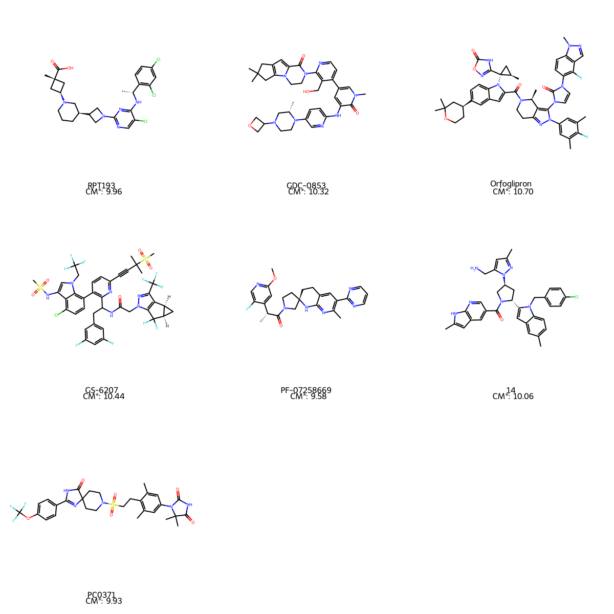
The native visualisation of RDKit is not very clear. Let’s try something with Matplotlib
#define molecular visualisation function:

#from rdkit.Chem.Draw import MolsToGridImage


def grid_mols_with_annotation(mols, labels, sub_img_size=500, mols_per_row=3, title="", annotation_size=15, title_size=25, y_offset=-5):
    """Annotates a MolsToGridImage given a set of labels for each mol with better font size options and title"""

    img = Draw.MolsToGridImage(mols, molsPerRow=mols_per_row, maxMols = len(mols), subImgSize=(sub_img_size, sub_img_size), returnPNG=False)

    fig, ax = plt.subplots(figsize=(40,40))
    plt.title(title, fontsize=title_size)
    text_pos = (sub_img_size/2, sub_img_size+y_offset)
    pos_ctr = 0
    plt.axis("off")
    for cmpd_text in labels:
        plt.annotate(cmpd_text, text_pos, fontsize=annotation_size, horizontalalignment='center')
        pos_ctr += 1
        text_pos = (text_pos[0]+sub_img_size, text_pos[1])
        if (pos_ctr % mols_per_row) == 0:
            text_pos = (sub_img_size/2, text_pos[1] + sub_img_size)

    ax.imshow(img, origin="upper")
    plt.show()
mols_ = [Chem.MolFromSmiles(i) for i in data['SMILES']]

labels_ = [(f'{row[0]} \n CM*: {row[3]:.2f}')
           for ind, row in data.iterrows()]
grid_mols_with_annotation(mols_, labels_, annotation_size=40)
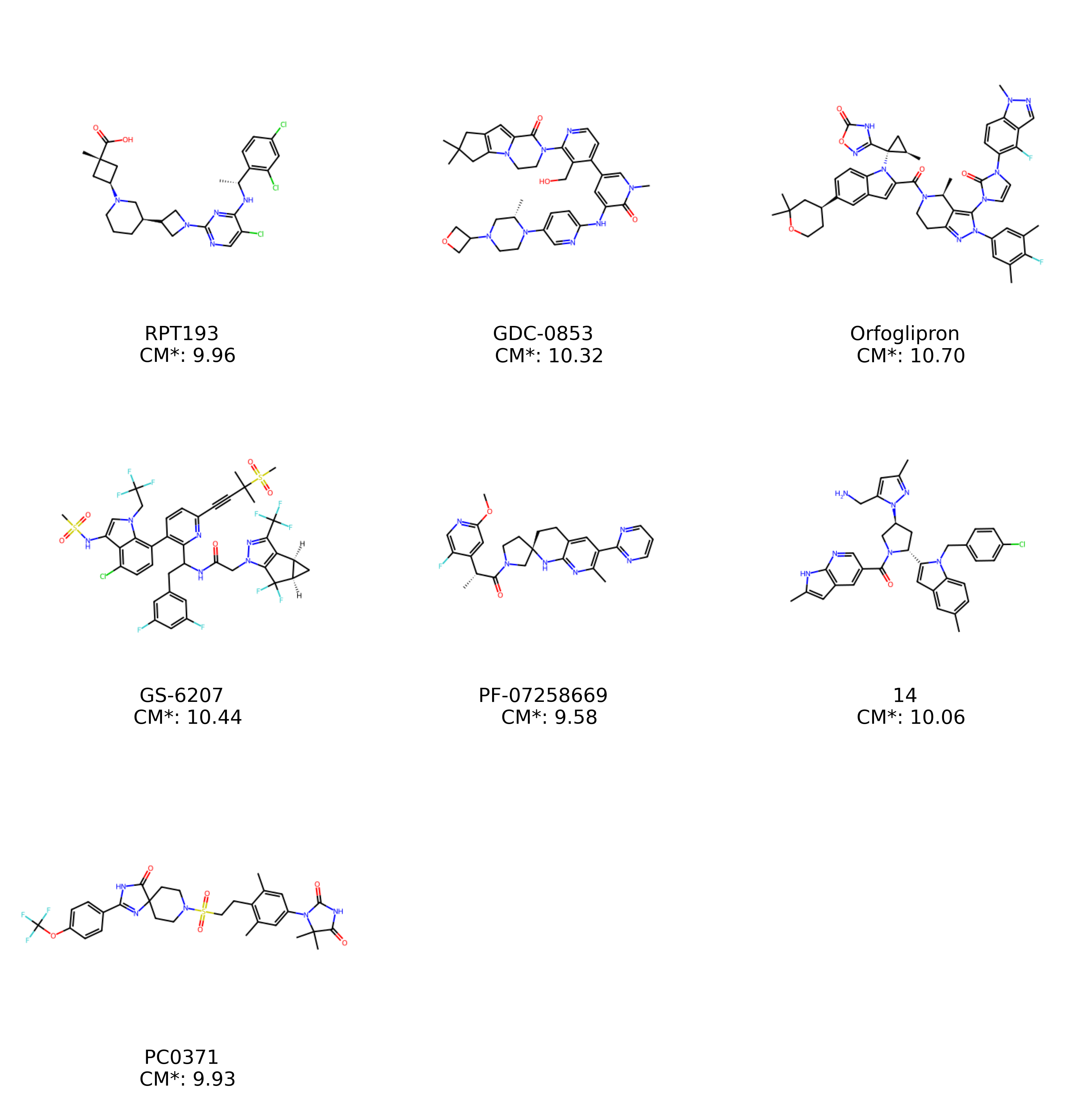
Ahhhh! Much better
OK, now for added context let’s see where on the CM* vs CSe plot these molecules lie. I will use a set of 5000 compounds consisting of APIs and their intermediates harvested from publicly available data and anonymised.
#load the anonymised data

anon_data = pd.read_csv('mock_complexity_data.csv')

anon_data.head()
| CM_py | CM_Star_py | CSe | |
|---|---|---|---|
| 0 | 117.687757 | 9.055736 | 4.651084 |
| 1 | 137.239575 | 9.340536 | 4.748940 |
| 2 | 41.664949 | 7.306858 | 3.459432 |
| 3 | 272.170352 | 10.090550 | 4.860877 |
| 4 | 52.074573 | 7.522323 | 3.906891 |
#visualisation

fig, ax = plt.subplots(figsize=(8,6))

ax.scatter(anon_data['CM_Star_py'],
           anon_data['CSe'],
           color = 'gray',
           s=0.5, alpha=0.1)

ax.scatter(data['CM*'],
           data['Cse'],
          s=30)

ax.set_xlim(4, 12)
ax.set_ylim(2, 6)
ax.set_xlabel('CM*: -> More complex features')
ax.set_ylabel('CSe: -> More diverse atom types')

ax.set_title('CM* vs CSe', loc='left', pad=10)
plt.show()
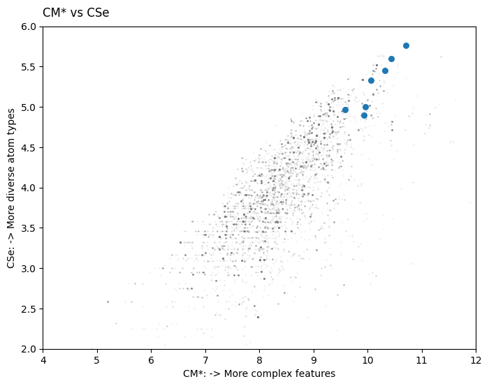
This compounds reside on the upper right region of the graph, showing very high degree of molecular complexity. CM* is a measure of ‘more complex’ features or more ‘complex features’, and CSe is a measure of the diversity of atom types.
The above is great. Now let’s see which atoms contribute most to the molecular complexity of each of the compounds we are looking at.
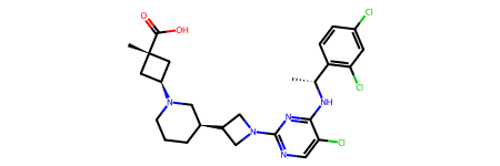
Let’s work with a single molecule as an example
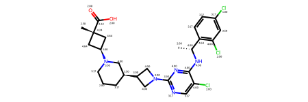
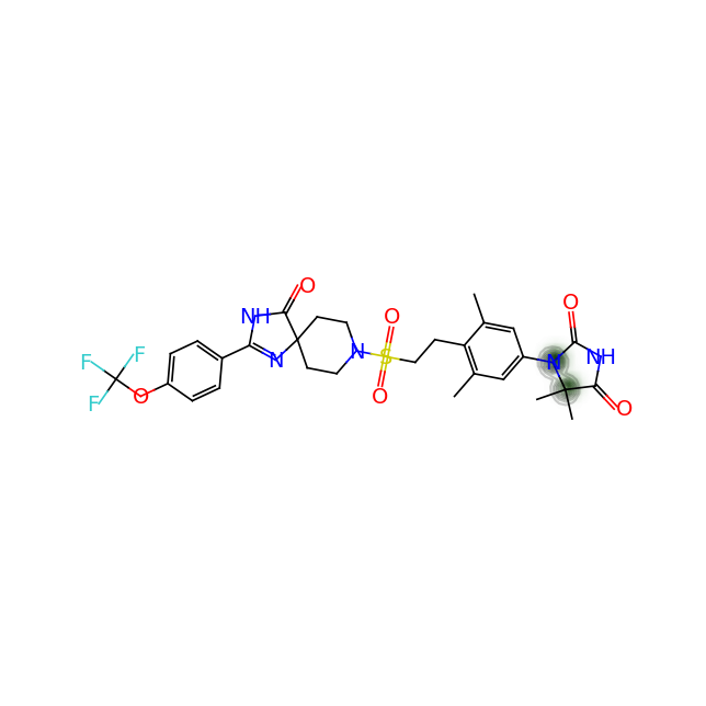
mol = Chem.MolFromSmiles(data['SMILES'][0])
mol
We can get the atom complexities using existing code
# get atom types for each atom in the molecule
atoms = [(atom.GetIdx(), get_atom_type(atom)) for atom in mol.GetAtoms()]

# create dict with neighbors of each atom
neighbors = {
    atom: [atoms[neighbor.GetIdx()] for neighbor in mol.GetAtomWithIdx(atom[0]).GetNeighbors()]
    for atom in atoms
}

atom_paths = _collect_atom_paths(neighbors)

cas = np.zeros(len(atom_paths))
for i, paths in enumerate(atom_paths):
    total_paths = len(paths)
    pi = fractional_occurrence(paths)
    cas[i] = -np.sum(pi * np.log2(pi)) + np.log2(total_paths)
We can then map the atom complexities on the molecule
for atom_ind, ca in enumerate(cas):
    mol.GetAtomWithIdx(atom_ind).SetProp('atomNote', f'{ca:.2f}')

mol
And use a heatmap to understand which atoms contribute most to the molecular complexity of each structure
fig = SimilarityMaps.GetSimilarityMapFromWeights(mol, cas, alpha=0.1)#, colorMap='Greys_r', contourLines=5)
#'gist_gray', 'Greys', 'gist_yarg','spring','Greys_r can also be used
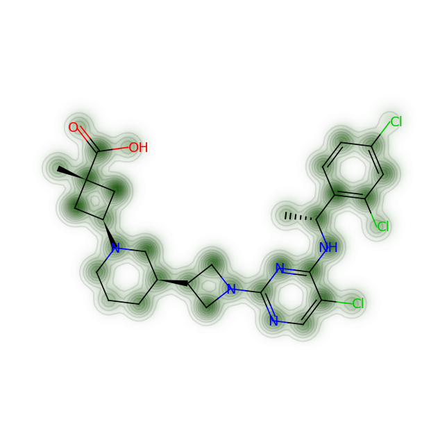
The above visualisation is not ideal. There is still ambiguity when it comes to understanding which molecules contribute most. We can normalise the values of the atom complexity array, and get a copy of that array with values >80% and everything else set to 0.
cas
array([2.        , 4.        , 4.64385619, 4.        , 2.        ,
       4.        , 4.        , 4.        , 3.5       , 3.        ,
       4.        , 3.        , 3.5       , 4.        , 3.5       ,
       3.        , 4.64385619, 4.24385619, 2.50325833, 4.24385619,
       2.        , 2.        , 4.64385619, 3.169925  , 2.        ,
       3.169925  , 4.        , 3.169925  , 3.169925  , 4.        ,
       2.        , 3.169925  , 3.169925  , 3.169925  , 1.        ,
       3.5       ])
cas_norm = (cas-np.min(cas))/(np.max(cas)-np.min(cas))

cas_norm
array([0.27443454, 0.82330362, 1.        , 0.82330362, 0.27443454,
       0.82330362, 0.82330362, 0.82330362, 0.68608635, 0.54886908,
       0.82330362, 0.54886908, 0.68608635, 0.82330362, 0.68608635,
       0.54886908, 1.        , 0.89022618, 0.41254601, 0.89022618,
       0.27443454, 0.27443454, 1.        , 0.59550237, 0.27443454,
       0.59550237, 0.82330362, 0.59550237, 0.59550237, 0.82330362,
       0.27443454, 0.59550237, 0.59550237, 0.59550237, 0.        ,
       0.68608635])
cas_processed = [value if value>=0.8 else 0 for value in cas_norm]
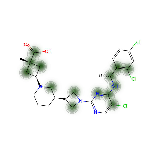
Now do the heatmap visualisation with the processed values
fig = SimilarityMaps.GetSimilarityMapFromWeights(mol, cas_processed, alpha=0.2)#, colorMap='Greys_r', contourLines=5)

Much better - the added advantage of the above method is that you can tune the threshold as well
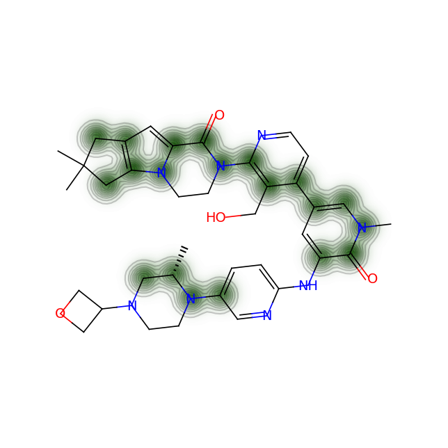
Let’s do it for all the molecules in our collection:
for smile in data['SMILES']:

    mol = Chem.MolFromSmiles(smile)

    # get atom types for each atom in the molecule
    atoms = [(atom.GetIdx(), get_atom_type(atom)) for atom in mol.GetAtoms()]

    # create dict with neighbors of each atom
    neighbors = {
        atom: [atoms[neighbor.GetIdx()] for neighbor in mol.GetAtomWithIdx(atom[0]).GetNeighbors()]
        for atom in atoms
    }

    atom_paths = _collect_atom_paths(neighbors)

    cas = np.zeros(len(atom_paths))
    for i, paths in enumerate(atom_paths):
        total_paths = len(paths)
        pi = fractional_occurrence(paths)
        cas[i] = -np.sum(pi * np.log2(pi)) + np.log2(total_paths)

    cas_norm = (cas-np.min(cas))/(np.max(cas)-np.min(cas))

    cas_processed = [value  if value>=0.8 else 0 for value in cas_norm]

    fig = SimilarityMaps.GetSimilarityMapFromWeights(mol, cas_processed, alpha=0.2)
    #fig = SimilarityMaps.GetSimilarityMapFromWeights(mol, cas_processed, colorMap='Greys_r', contourLines=5)
Let’s compare the above figures with the attributed complexity hotspots from the LinkedIn post:
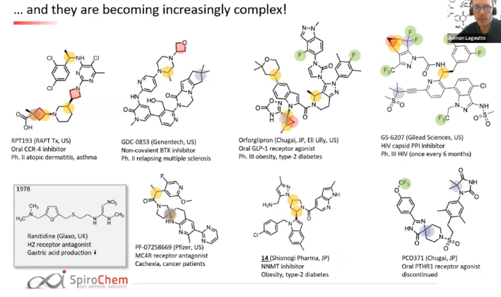
Here are a few examples:
-
For RPT193, the cyclobutane and azetidine rings are obvious complexity hotspots. The calculation above highlights an additional region between the pyrimidine and appended chain with the dichlorophenyl ring.
-
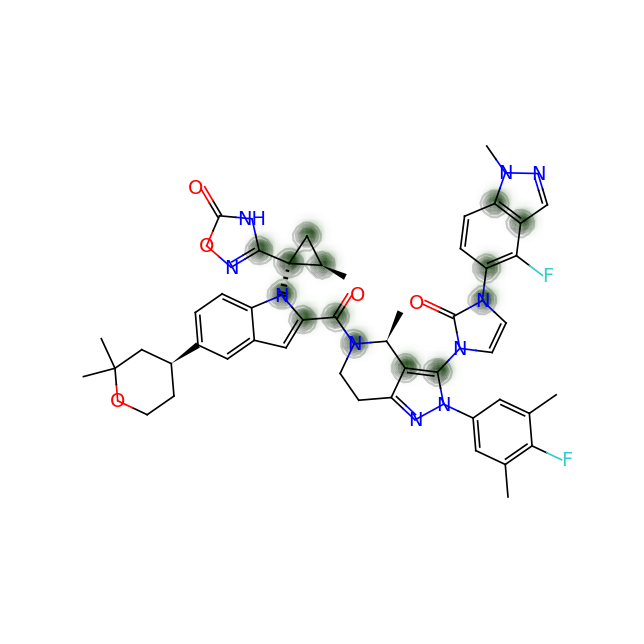
For GDC-0853: Only the gem-dimethyl motif and the oxatane ring are highlighted in the post above. However, the calculation shows a more extened region spaning from the pyridone ring and covering the whole 6-5-5 ring system on one end of the molecule.
-
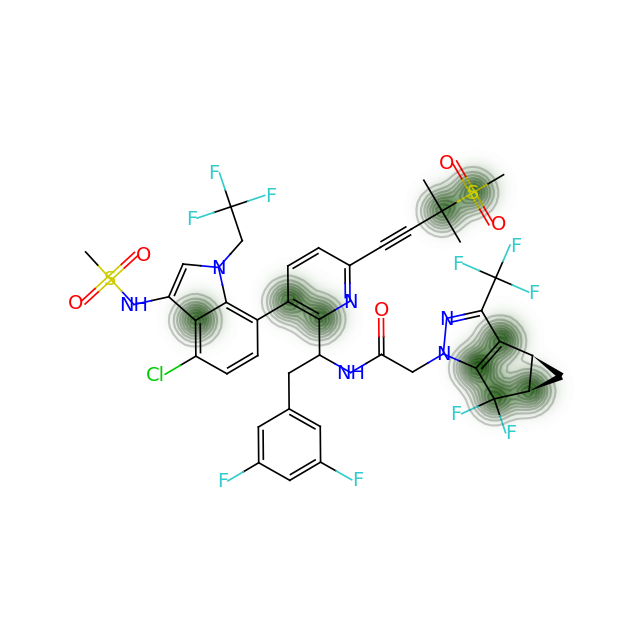
For GS-6207: Again very arbitrary points of the compound are highlighted. On the other hand the calculation shows us that there are non-obvious complexity hotspots around the gem-dimethyl groups next to the methane-sulfonate group, the cyclopropapyl and gem-difluoro area as well as the junction of the indole and the ortho-and meta- carbon atoms of the pyridine ring.
In conclusion, molecular complexity is a quantity that can be quantified in different ways and can give us a better graps of the synthetic challenge that a compound may pose. I would strongly recommend to avoid using the term without any calculations and their associated caveats to refrain from generalities. Especially since with Python, RDKit and some personal drive, one can get numbers that may be of actual use.